One Motor

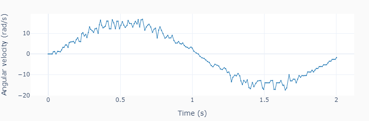
This example code shows how to precisely apply a time-based excitation (in this case a sine wave) to a single motor. Keeping track of the current execution time is the key to achieving that. The motor speed is calculated as the derivative of the tacho angular position output.

""" onemotor.py

Run one motor with a sinusoidal speed input.

Setup:
    Connect one large motor to port 'A'

"""
# Importing modules and classes
import time
import numpy as np
from pyev3.utils import plot_line
from pyev3.brick import LegoEV3
from pyev3.devices import Motor

# Defining parameters (for one motor)
T = 2  # Period of sine wave (s)
u0 = 80  # Motor speed amplitude (%)
tstop = 2  # Sine wave duration (s)

# Pre-allocating output arrays
t = []
theta = []

# Creating LEGO EV3 objects
ev3 = LegoEV3()
motor = Motor(ev3, port='A')

# Initializing motor
motor.outputmode = 'speed'
motor.output = 0
motor.reset_angle()
motor.start()

# Initializing current time stamp and starting clock
tcurr = 0
tstart = time.perf_counter()
# Running motor sine wave output
while tcurr <= tstop:
    # Getting current time (s)
    tcurr = time.perf_counter() - tstart
    # Assigning current motor sinusoidal
    # output using the current time stamp
    motor.output = u0 * np.sin((2*np.pi/T) * tcurr)
    # Updating output arrays
    t.append(tcurr)
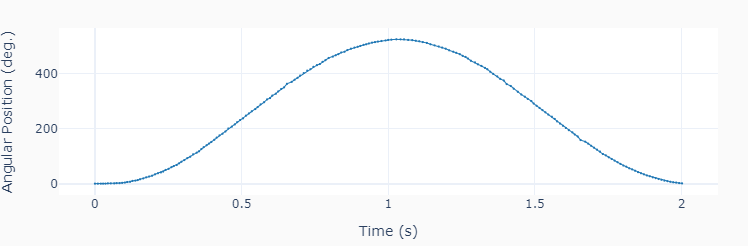
    theta.append(motor.angle)
# Stopping motor and closing brick connection
motor.stop()
ev3.close()

# Calculating motor angular velocity (rad/s)
w = 2*np.pi/360 * np.gradient(theta, t)

# Plotting results
plot_line([t], [theta], yname=['Angular Position (deg.)'], marker=True)
plot_line([t], [w], yname=['Angular velocity (rad/s)'], marker=True)